An R Package for Positional Accuracy Improvement of Vector Maps • mapAI

The mapAI package is designed to provide a comprehensive and accessible PAI (positional accuracy improvement) framework for vector geospatial data.

Overview

The mapAI package provides a comprehensive and accessible framework for Positional Accuracy Improvement (PAI) of vector geospatial data. This package’s main contributions are:

the unification of a set of PAI methods from classical adjustments to statistical and machine learning algorithms, within a framework engineered to modify the geometry of spatial features;
the application of modern best practices regarding predictive accuracy assessment using;
the integration of distortion analysis into the PAI workflow, providing powerful diagnostics.

Installation

You can install the development version of mapAI from GitHub using the pak package:

# install.packages("pak")
pak::pak("kvantas/mapAI")

Core Workflow: A Complete Example

This example demonstrates the primary workflow. We will first generate a synthetic dataset representing a distorted map and then use the package’s functions to correct it.

1. Load Libraries and Create Demo Data

We begin by using create_demo_data() to generate a test case with complex, noisy distortions.

library(mapAI)
library(sf)
#> Linking to GEOS 3.13.0, GDAL 3.8.5, PROJ 9.5.1; sf_use_s2() is TRUE
library(ggplot2)

# Generate a shapefile and a GCPs CSV with complex noisy distortions
# The function returns a list containing the paths to these new files.
demo_files <- create_demo_data(type = "complex", seed = 42)
#>    -> Homologous points saved to: /var/folders/yh/kq6cp_457lg059f3l02r57s80000gn/T//RtmpUC7CRv/demo_gcps.csv
#>    -> Distorted map saved to: /var/folders/yh/kq6cp_457lg059f3l02r57s80000gn/T//RtmpUC7CRv/demo_map.shp

2. Read Data and Train a Model

We load the generated files and train a Generalized Additive Model (gam), which is ideal for capturing the smooth, non-linear distortions present in the demo data.

# Load the homologous points (GCPs) and the distorted vector map
gcp_data <- read_gcps(gcp_path = demo_files$gcp_path)
map_to_correct <- read_map(shp_path = demo_files$shp_path)
#> Reading layer `demo_map' from data source 
#>   `/private/var/folders/yh/kq6cp_457lg059f3l02r57s80000gn/T/RtmpUC7CRv/demo_map.shp' 
#>   using driver `ESRI Shapefile'
#> Simple feature collection with 30 features and 1 field
#> Geometry type: LINESTRING
#> Dimension:     XY
#> Bounding box:  xmin: -0.3737642 ymin: -4.996873 xmax: 102.7303 ymax: 115.3157
#> Projected CRS: WGS 84 / Pseudo-Mercator

# Train the GAM model using the GCPs
gam_model <- train_pai_model(gcp_data, pai_method = "gam")
#> Training 'gam' model...

3. Apply Correction and Visualize

We apply the trained model to our distorted grid. The resulting plot, which overlays the corrected grid on the original, provides a clear visual confirmation of what the model does to the distorted map.

# Apply the model to the distorted map
corrected_map <- apply_pai_model(gam_model, map_to_correct)
#> Applying PAI model to map features...
#> Correction complete.

# For easy plotting, add a 'status' column and combine the maps
map_to_correct$status <- "Original (Distorted)"
corrected_map$status <- "Corrected"
comparison_data <- rbind(map_to_correct[, "status"], corrected_map[, "status"])

# Create the final comparison plot
ggplot(comparison_data) +
  geom_sf(aes(color = status, linetype = status), fill = NA, linewidth = 0.7) +
  scale_color_manual(name = "Map Status", values = c("Original (Distorted)" = "grey50", "Corrected" = "#e41a1c")) +
  scale_linetype_manual(name = "Map Status", values = c("Original (Distorted)" = "dashed", "Corrected" = "solid")) +
  labs(title = "Positional Correction of a Distorted Grid",
       subtitle = "Overlay of original (dashed) and mapAI-corrected (solid) geometries") +
  theme_minimal()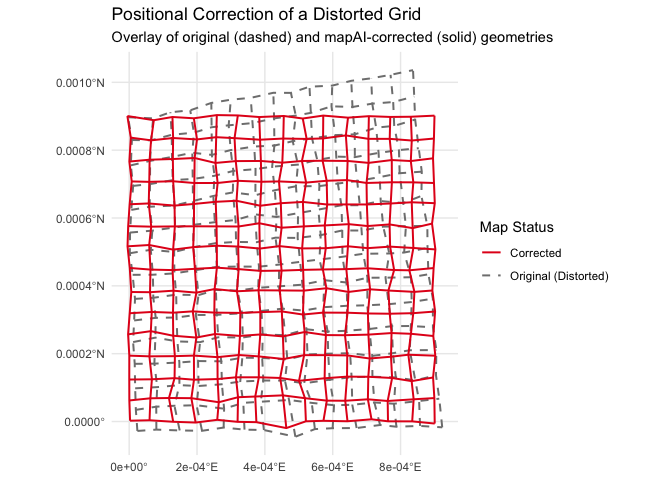

From Correction to Explanation: Advanced Distortion Analysis

A key challenge with data-driven models is understanding what they have learned. mapAI directly addresses this by providing tools to “open the black box” and analyze the properties of the learned transformation.

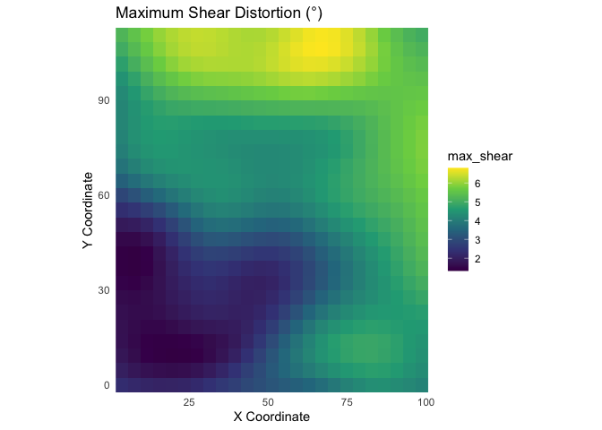
4. Quantify and Visualize the Distortion Field

The analyze_distortion() function computes local distortion metrics across the map space. This allows us to move from a simple visual assessment to a quantitative map of the distortion.

# 1. Create a grid of points for analysis using the pipe (%>%)
library(magrittr)
analysis_points <- sf::st_make_grid(gcp_data, n = c(25, 25)) %>%
  sf::st_centroid() %>%
  sf::st_sf()

# 2. Analyze the distortion using our trained GAM model
distortion_results <- analyze_distortion(gam_model, analysis_points)

# 3. Plot the distortion surfaces
plot_area <- plot_distortion_surface(
  distortion_results, metric = "log2_area_scale", diverging = TRUE
) + labs(title = "Areal Distortion (log2σ)")

plot_shear <- plot_distortion_surface(
  distortion_results, metric = "max_shear"
) + labs(title = "Maximum Shear Distortion (°)")

# Show the plots
plot_area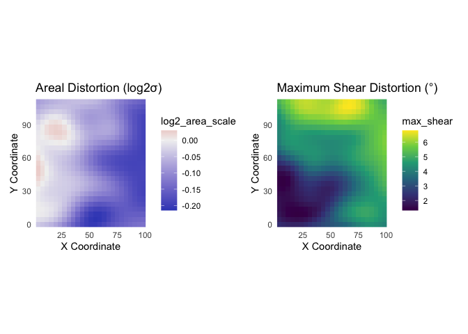

plot_shear

mapAI